A Simple Guide to Power Analysis

What is statistical power?

Statistical power is the probability that a study detects an effect when that effect actually exists.

Imagine a diagnostic test for a fake disease called cucumberitis. If the test frequently returns a negative result when the patient is sick, it has a high false-negative rate. An underpowered experiment has an analogous problem: a real effect can be present even when the statistical test fails to detect it.

Low power makes negative results difficult to interpret. Did the manipulation fail, or was the study simply too noisy to reveal its effect? A power analysis helps us distinguish those possibilities before collecting data. Two of its most important inputs are the effect size we want to detect and the sample size we plan to collect.

Why do we run weak tests?

“I can’t do a power analysis because I have no idea what the effect size is. If I knew the effect size, I wouldn’t have to run the study in the first place!”

This is a common objection, and underlies why many still don’t do power analyses—but it turns out, we know much more than we think we do. For instance, here is a distribution of effect sizes from a meta-analysis of meta-analyses in social psychology collecting effect sizes across ~25,000 studies over 100 years in diverse research areas (credit to Jake Westfall for this analysis):

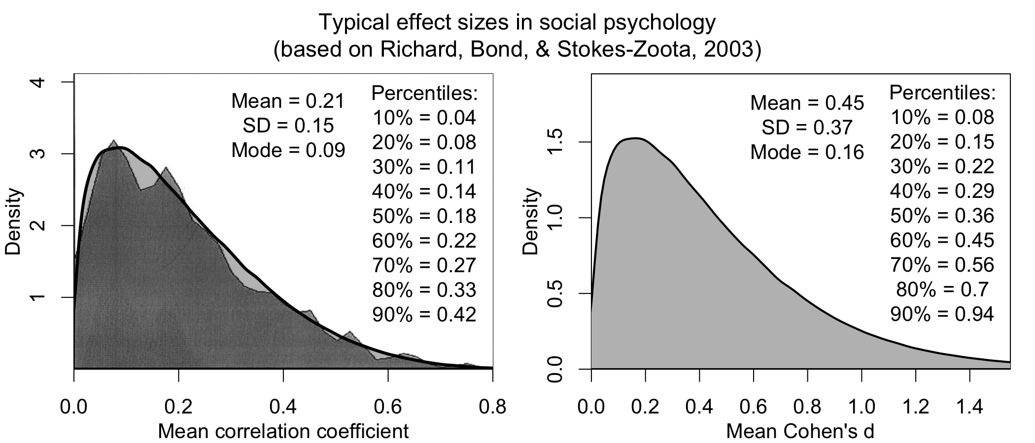
When prior evidence is sparse, broad empirical distributions can still constrain our expectations. In many areas of social psychology, reported standardized effects cluster in the small-to-moderate range, and publication bias may make those reports optimistic. This does not imply that every new effect is probably d = .3, but it gives us a more defensible starting range than assuming an arbitrarily large effect.

Moreover, Joe Simmons has run some extremely helpful, large (N ~ 700) studies on the effect sizes of very simple questions. Consider a classic psych question: Do smokers think that smoking is less risky than non-smokers? What do you think the effect size is for this? It turns out to be ~.3. How about the likelihood that someone who likes eggs eats more egg salad? The effect size is ~.5.

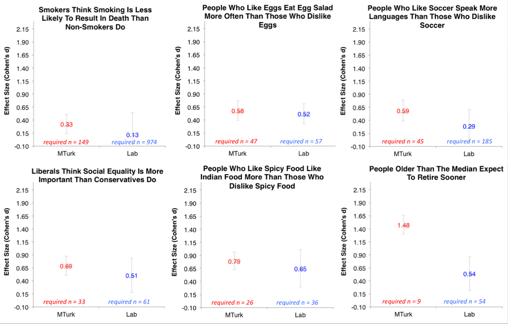
The upshot is that even seemingly obvious relationships can have small-to-moderate effect sizes. A useful power analysis should therefore consider several plausible effects. If a design works only when the effect is unusually large, that is itself important information.

Trust your priors more than your pilots

Often, we’ll do a smaller pilot study, and use the effect size estimates from that to do power analyses. This is probably not a good idea, unless your pilots are very large, mostly because getting tight bounds on effect sizes requires very large samples, e.g., N > 3000 (see below, courtesy of Uri Simonsohn) .

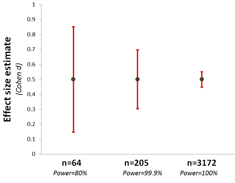
This means that your pilot tells you less than you think about how big your effect probably is.

Implementing a simple, simulation-based power analysis in R

Hopefully you are vaguely convinced that you should try power analyses. Here is my favorite way to do them.

The intuition is simple: given an effect and a sample size, we want to know how often our analysis would detect the effect. We can generate artificial data in which the effect is present, analyze those data, and repeat the process many times. The proportion of simulations that detect the effect estimates our statistical power.

Toy example: Does eating cucumbers make you less thirsty? Let’s assume a standardized mean difference of d = .5. What is our likelihood of detecting it in a typical psychology sample at p < .05? Suppose 30 people were given cucumbers, 30 were not, and everyone rated their thirst from 0 to 10.

The no_cucumber group has a mean thirst rating of 5. Because the standard deviation is 1, a standardized effect of d = .5 corresponds to a mean of 4.5 in the cucumber group. Let’s generate these samples and run a t-test:

set.seed(2026)

cucumber <- rnorm(n = 30, mean = 4.5, sd = 1)
no_cucumber <- rnorm(n = 30, mean = 5, sd = 1)

t.test(cucumber, no_cucumber)

In this instance, there was enough signal in the randomly generated data that I could find it:

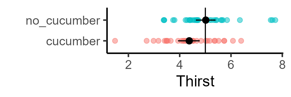
One simulated experiment is not enough because a new random sample can produce a different result. Instead, we can generate and analyze 1,000 datasets, then collect their p-values:

set.seed(2026)

test_pvalues <- replicate(1000, {
  cucumber <- rnorm(n = 30, mean = 4.5, sd = 1)
  no_cucumber <- rnorm(n = 30, mean = 5, sd = 1)

  t.test(cucumber, no_cucumber)$p.value
})

Here is the distribution of p-values. Red shows the mean p-value, and blue shows p = .05. Because we generated every dataset with a real effect, the values above .05 are false negatives: experiments that did not detect the effect we put there.

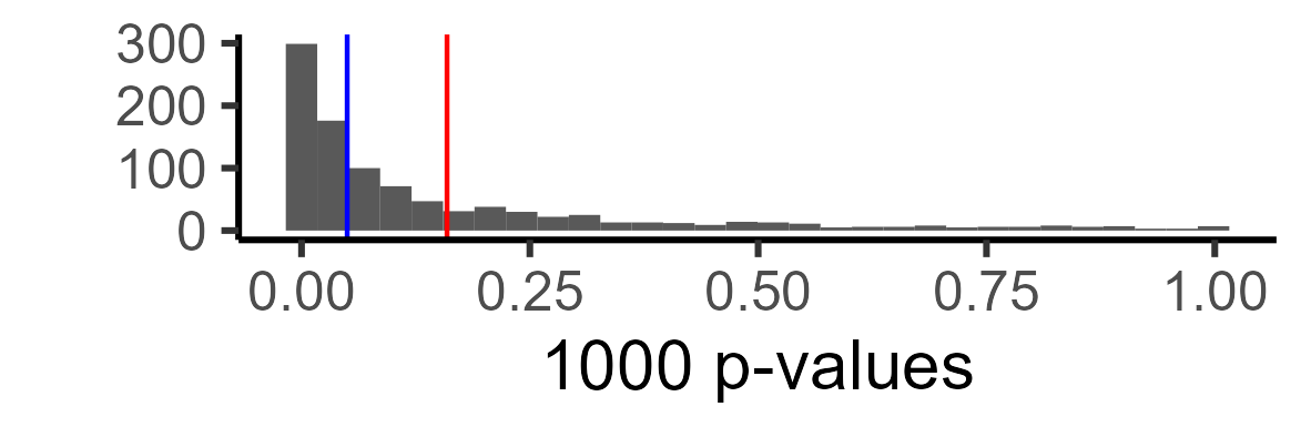
Our estimated power is the proportion of simulated experiments in which the test detected the effect:

mean(test_pvalues < 0.05)

Setting the random seed makes this example reproducible. The result will be close to, but not exactly equal to, the theoretical power because it is estimated by simulation. We can run more simulations for a more precise estimate or change the assumptions to see how power responds. What happens, for example, if the standard deviation is 2 rather than 1?

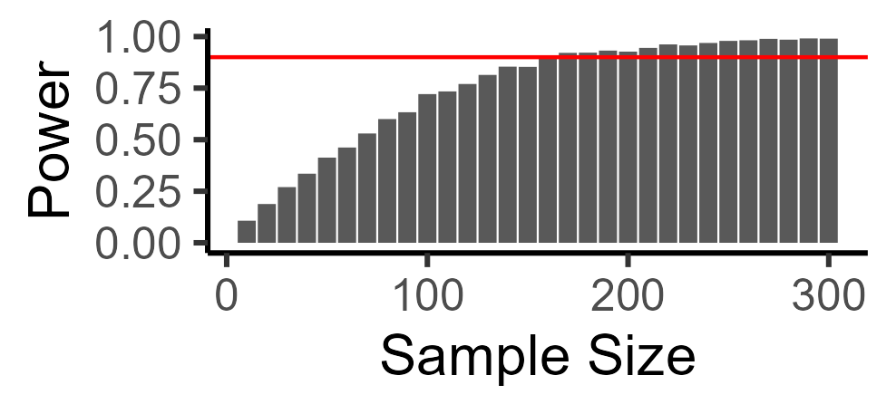
We can also ask what sample size would give us good power, such as 90%. I find simulations intuitive, so we can estimate power across a range of candidate sample sizes. In this setup, the required total sample is approximately 170:

Here is the code:

set.seed(2026)

estimate_power <- function(sample_size, simulations = 1000) {
  p_values <- replicate(simulations, {
    cucumber <- rnorm(n = sample_size / 2, mean = 4.5, sd = 1)
    no_cucumber <- rnorm(n = sample_size / 2, mean = 5, sd = 1)

    t.test(cucumber, no_cucumber)$p.value
  })

  mean(p_values < 0.05)
}

sample_sizes <- seq(50, 300, by = 10)
power_estimates <- vapply(sample_sizes, estimate_power, numeric(1))

The same method extends naturally to more complicated analyses: generate data under your assumptions, fit the model you plan to use, and record how often it detects the target effect. For complex or computationally expensive designs, an established power-analysis package may be more convenient.

Power matters

I wrote this because I have run dozens of studies with thousands of participants that, in retrospect, told me much less than I thought they did. In the example above, a standard design with 30 participants per condition has only about .5 power. A negative result would therefore leave two live possibilities: the effect was absent, or the study was too noisy to detect it.

Power increases nonlinearly with sample size. Recruiting more participants makes a real effect easier to detect and usually narrows our uncertainty, but a nonsignificant result still does not establish that the effect is exactly zero. Answering that stronger question requires examining confidence intervals or using tools such as equivalence tests.

I could have learned much more from fewer, better-powered studies. Better designs would not have told me with certainty which effects were real, but they would have produced more precise estimates and made negative findings substantially more informative.

For more info on why this matters for psychology research, check out the article by Paul Meehl in my list of favorite articles, or check out Uri, Joe, and Jake’s posts above. Data Colada in particular has a lot of useful write-ups on this.

---